Boolean Algebra - A Form of Logic

Let's talk about logic. For Boolean algebra, it is logic in the form of algebra. True and false are represented by 1 and 0. The “or” and “and” correspond to addition and multiplication. In short, it takes logic and its operations and laws and transforms it to a more familiar language, algebra. I think Boolean algebra makes logic easier.

In this post, I will go over the symbols, properties, and laws of Boolean algebra. I will compare it to symbolic logic and regular algebra. I will briefly discuss how implication (IF-THEN) can be converted to Boolean algebra. Then I will show using Boolean algebra that four common arguments are valid arguments.

Symbolic Logic	Boolean Algebra
True False Statement x X’ X˄Y X˅Y X→Y	1 0 X X’ or (1-x) XY or X∙Y X+Y N/A

Properties and Laws of Boolean algebra

1.  Idempotent laws

a.       X+X=X

b.      XX=X

2. Bound laws

a.       X+1=1

b.      X0=0

3. Absorption laws

a.       X+XY=X

b.      X(X+Y)=X

4. Involution laws

a.       (X’)’=X

5. 0 and 1 laws

a.       0’=1

b.      1’=0

6. De Morgan's laws for Boolean algebra

a.       (X+Y)’=X’Y’

b.      (XY)’=X’+Y’

The laws and properties for addition and multiplication can be used as well including commutative, associative, and distributive properties.

1. Commutative property

a.       X+Y=Y+X

b.      XY=YX

2. Associative property

a.       (X+Y)+Z=X+(Y+Z)

b.      (XY)Z=X(YZ)

3. Distributive property

a.       X(Y+Z)=XY+XZ

However, unlike regular algebra, you can do addition over multiplication as well.

X+YZ=(X+Y)(X+Z)

Boolean algebra is the language of logic, so you have both the distribution of conjunction (and) and disjunction (or).

This also means that X implies Y can be converted to Boolean algebra. From logic, we know the tautology, implication to disjunction.

(X→Y)↔(X’˅Y)

So X→Y would be X’+Y or (1-X)+Y in Boolean algebra. This will be useful for the next section.

Four Common Valid Arguments

If p, then q P Thus, q

If p, then q Not q Thus, not p

If p, then q If q, then r Thus, if p, then q

P or Q Not P Thus, Q

Valid argument can found using the laws and properties of Boolean algebra to reach the conclusion. Valid arguments assumes the premises are true. This also can be used. Remember, an argument is valid when both the premises and the conclusion are true. With the assumption that the premises are true, if the conclusion is false or unknown, then the argument is invalid.

First argument

If p, then q p

(1-p)+q using implication to disjunction p=1 since assumption of true premises

(1-p)+q

(1-1)+q

0+q

Thus, q

An argument is a large conditional statement where the “if” is a line of premises connected by “AND”.

IF p1p2p3…,THEN conclusion.

Another way

((1-p)+q)p

p(1-p)+pq

0+pq

pq

1q since p=1

Thus, q

Second argument

If p, then q Not q

(1-p)+q using implication to disjunction 1-q=1 since assumption of true premises

1-q=1

q=0

1-p+q

1-p+0

1-p

Thus, not p.

Third argument

If p, then q If q, then r

(1-p)+q or p’+q using implication to disjunction (1-q)+r or q’+r using implication to disjunction

(p’+q)(q’+r)

p’q’+p’r+qq’+qr

p’q’+p’r+0+qr

p’q’+p’r+qr

p’q’+p’r+p’r+qr

p’(q’+r)+r(p’+q)

p’1+r1

Thus, p’+r

Fourth argument

P or Q Not P

p+q 1-p

1-p=1

p=0

p+q

0+q

Thus, q.

For more on logic, check out my youtube channel. If you have any questions or blog ideas, you can e-mail me at jdmathguy@gmail.com

System of Equations and Matrices

Let's talk about solving a system of equations using matrices, specifically Gaussian Elimination and Gauss-Jordan Elimination. In the first example, I will show the "in-between" steps using the row transformations. In the second example, I will not show the "in-between" steps, use the Gauss-Jordan Elimination method. Also it will a system of 4 equations with 4 unknowns.

Example 1: Solve using Gaussian Elimination

If you are able, always check your answer by plugging in what you found. If it is true for all, then it is a solution.


Example 2: Solve using Gauss-Jordan Elimination

First, convert the system of equations to a matrix. Then with each step, apply the row transformations. With the Gauss-Jordan method, you want to keep going until you get the identity matrix on the left-hand side. The identity matrix has a diagonal of 1's and the rest are zeroes. Gauss-Jordan Elimination is like Gaussian Elimination, but it goes a little further.

For more on matrices, check out my youtube channel. If you have any questions or blog ideas, you can e-mail me at jdmathguy@gmail.com

A Method for Factoring Polynomials: OI-Box Method

Let's talk about factoring polynomials. The method I'm going to show you is almost universal. It is a combination of the product-sum method, OI method, and the box method. This method of factoring can factor 2 terms (difference of squares), 3 terms (A=1), 3 terms (A doesn't =1), and 4 terms.

I call this method of factoring, the OI-box method. It is a variation on the OI method. If you are curious about the OI method, check out my recent YouTube video: OI method. It uses the Outer and Inner of FOIL. This method does the same. I'll explain the steps of the method first. Second, I will show a flowchart related to the method. Then I will show you some examples.

1. The Steps of Method

Step 1: Identify the number of terms and type.

Step 2: Apply the product-sum if necessary.

• Set-up. Put AC on the top and B on the bottom. 
• Find the left and the right by asking two questions
• What product equals AC?
• What sum equals B

Step 3: Apply the OI-box method. The solutions found in step 2 are the outer and inner or the O-I in FOIL.

• Set-up. Rows as O-I and Columns as F-L in FOIL
• Find the squares either by GCF of row and column or missing factor within a row or column.
• If needed, put negative only in the L-column.

Step 4: Take the diagonals found in step 3 and use them as factors.

Note: For trinomials (Ax²+Bx+C), they are factorable when B²-4AC equals a square (i.e. 0, 1,4,9,...). If not, it is prime.

2. Flowchart of the Method

3. 5 Examples using the Method

A. Factor polynomial with 4 terms

B. Factor trinomial (3 terms) with A equals 1

C. Factor trinomial (3 terms) with A doesn't equal 1

D. Factor perfect square trinomial (3 terms)

E. Factor a difference of squares (2 terms)

A. Example 1

B. Example 2

C. Example 3

D. Example 4

E. Example 5

Conclusion

For a method of factoring, it covers a wide variety of scenarios. The method cannot be used with a difference or sum of cubes, or when you have a difference of squares with 4 terms. Nonetheless this method of factoring can be very useful.

How Rational Expressions are like Fractions

Let's talk about rational expressions. When it comes to rational expressions, you need to know two things: factoring polynomials and fractions. It is important to know fractions because the steps for doing an operation with rational expressions is similar to an operation done between two fractions. Factoring is important because you can only cancel out factors with factors just like fractions.

In this post, I will compare the operations with fractions with rational expressions. I will line them up side by side. They should be the same if you set x equal to zero.

1. Simplifying rational expressions is like simplifying fractions

Note: you can only cancel out factors with factors.

2. Multiplying rational expressions is like multiplying fractions


Note: you can cancel within the same fraction or diagonally. It is always a factor of a numerator with the same factor in the denominator.

3. Dividing rational expressions is like dividing fractions





















Note: you have to first k-c-f it before you cancel things out. K-C-F stands for keep it, change it, and flip it.

4. Adding and subtracting rational expressions is like adding and subtracting fractions

Note: When you are adding and subtracting fractions, you have to find the LCD and equivalent fractions first to add the numerators. The denominators have to be the same. You don't cancel anything till its one fraction.

Simplifying rational expressions can be difficult, but remember they are just like fractions.

Deriving the Pythagorean Trigonometric Identities

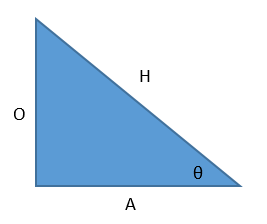
Let's talk about the Pythagorean Trig Identities. Let's talk about how to derive the identities starting with Pythagorean theorem.

Using the Pythagorean theorem, we get:

Since sin(θ)=O/H and cos(θ)=A/H, then we get with some substitution:

Notice when you divide both sides of eqn. 1 by sin²θ.

Also see what happens when you take eqn. 1 and divide both sides by cos²θ.

So this is how you can derive the three Pythagorean Trigonometric Identities including…

Let's talk math.

Forms and Formulas for Lines

Let's talk about lines. In this post, I will talk about the various forms and formulas of lines. We will start with the slope formula.

We know with a line that a slope is constant. Its steepness is always the same.

This is the point-slope form. What if I take point-slope form, and plug in (0,b) , y-intercept, as the point.

Look, I got slope-intercept form.

Now, let's look at standard form:

Let's find the following
a. x-intercept (#,0)
b. y-intercept (0,#)
c. slope

a. x-intercept

For parts a and b, I can find the slope and y-intercept by solving for y, simplifying, and then comparing it to slope-intercept form.

Note on Forms and Formulas

The main difference between the two is a form describes all the points on the line. It describes the set of all points falling on the line. Whereas a formula results in a specified value given other values.

The slope formula is used to find the slope given two points. On the other hand, whether it is point-slope form, slope-intercept form, or standard form, it describes every point on the line. This is why the variables x and y are used. The form is true for every point (x,y) that satisfies the equation. (x,y) is varying on the line as the slope and a point are staying constant.

Review

For more on lines, check out my YouTube Videos.

Can a variance be negative?

Let's talk about a variance being negative. The other day I worked out a discrete probability distribution problem, and I got a negative variance. The variance is always positive. It would be zero if the data was all the same value. It should never be negative. 

In this post, I will show how I first did the problem. Then I’ll show why that the negative answer is incorrect, and how it happened.

Problem

Calls for a crisis hotline. The number of calls received per day at a crisis hotline is distributed as follows:

Number X	30	31	32	33	34
Probability P(x)	0.05	0.21	0.38	0.25	0.11

Find the mean, variance, and the standard deviation of the distribution.

(Problem #18 pg. 307 from Bluman, A. (2013). Elementary statistics (9th ed). New York, NY: McGraw-Hill)

Part 1: The work at first glance

Finding the mean

The mean is 32.2 using the rounding rule. This is correct.

Finding the variance

Obviously, you can’t get a negative variance, so I tried the exact mean, 32.16.

1.1 is the correct variance using the rounding rules.

Part 2: Finding the Error

The work is correct. It should not matter if you plug in the rounded or exact mean. The variance should still be positive. The issue comes up with the shortcut formula. When the regular formula is used for variance, it results in variance close to 1.0744 using the rounded mean, 32.2.

Note: the differences are always being squared resulting in either a zero or positive value. They are never negative. Because of this, variance is always positive. It should not matter if 32.16 or 32.2, but it does.

Using the regular formula with the rounded mean, it is pretty close to the variance using the exact mean. Here is the regular formula for variance using the exact mean:

It is the same as the shortcut formula as it should be. Notice with using the exact mean or the rounded mean, you still get 1.1 for your variance when using the rounding rules. But why is it when you use the rounded mean for the shortcut and regular formula you get two different answers with one being negative.

It is important here to look at how the shortcut formula is derived from the regular formula. Note that µ is a constant in the formula. 

The problem arises with the substitution. In order to make the substitution and combine like-terms, you are assuming that all µ’s are the same. If you use the rounded mean, the µ’s are not all the same. You will have unlike terms, so you will not able to combine them to simplify.

Notice the solution is the same one we found using the regular formula.

Conclusion

When you using the shortcut formula for calculating the variance for a discrete probability distribution, you have to be careful when you plug in a rounded mean. It is better to use the exact mean if possible, or to use a rounded mean closer to the exact. The question arises from this, “Does this happen with other shortcut formulas found in statistics?”

In case, if you worrying how to get the standard deviation, you just need to take the square root of the variance. By the way, variance should always be positive or equal to zero.